More Python (Stat/ML/Viz)

We continue our journey with Python. At the end of this week, you will be able to:

Statistical Models in Python

statsmodels is a Python package that provides functions for fitting statistical models, conducting statistical tests, and statistical data exploration.

Let’s read a data set from the list provided in this link. We use the mtcars data set in R package datasets.

import statsmodels.api as stat # allow to access easily to most of the functions
import statsmodels.formula.api as statf # allow to use formula style to fit the models
import pandas as pd
import numpy as np
import matplotlib.pyplot as plt

df = stat.datasets.get_rdataset("mtcars", "datasets").data # load data "mtcars" from the R package 'datasets'
print(df.info())
<class 'pandas.core.frame.DataFrame'>
Index: 32 entries, Mazda RX4 to Volvo 142E
Data columns (total 11 columns):
 #   Column  Non-Null Count  Dtype  
---  ------  --------------  -----  
 0   mpg     32 non-null     float64
 1   cyl     32 non-null     int64  
 2   disp    32 non-null     float64
 3   hp      32 non-null     int64  
 4   drat    32 non-null     float64
 5   wt      32 non-null     float64
 6   qsec    32 non-null     float64
 7   vs      32 non-null     int64  
 8   am      32 non-null     int64  
 9   gear    32 non-null     int64  
 10  carb    32 non-null     int64  
dtypes: float64(5), int64(6)
memory usage: 3.0+ KB
None
fit_olsregression = statf.ols("mpg ~ wt + cyl",data=df).fit()
print(fit_olsregression.summary())
                            OLS Regression Results                            
==============================================================================
Dep. Variable:                    mpg   R-squared:                       0.830
Model:                            OLS   Adj. R-squared:                  0.819
Method:                 Least Squares   F-statistic:                     70.91
Date:                Sat, 17 Aug 2024   Prob (F-statistic):           6.81e-12
Time:                        23:28:53   Log-Likelihood:                -74.005
No. Observations:                  32   AIC:                             154.0
Df Residuals:                      29   BIC:                             158.4
Df Model:                           2                                         
Covariance Type:            nonrobust                                         
==============================================================================
                 coef    std err          t      P>|t|      [0.025      0.975]
------------------------------------------------------------------------------
Intercept     39.6863      1.715     23.141      0.000      36.179      43.194
wt            -3.1910      0.757     -4.216      0.000      -4.739      -1.643
cyl           -1.5078      0.415     -3.636      0.001      -2.356      -0.660
==============================================================================
Omnibus:                        4.628   Durbin-Watson:                   1.671
Prob(Omnibus):                  0.099   Jarque-Bera (JB):                3.426
Skew:                           0.789   Prob(JB):                        0.180
Kurtosis:                       3.287   Cond. No.                         27.9
==============================================================================

Notes:
[1] Standard Errors assume that the covariance matrix of the errors is correctly specified.
pred_ols = fit_olsregression.get_prediction()
pred_ols.summary_frame().head()
                        mean   mean_se  ...  obs_ci_lower  obs_ci_upper
rownames                                ...                            
Mazda RX4          22.279145  0.601167  ...     16.885964     27.672326
Mazda RX4 Wag      21.465447  0.497629  ...     16.116566     26.814327
Datsun 710         26.252026  0.725244  ...     20.795395     31.708658
Hornet 4 Drive     20.380516  0.460267  ...     15.045648     25.715384
Hornet Sportabout  16.646958  0.775271  ...     11.161630     22.132285

[5 rows x 6 columns]
df["cyl"] = df["cyl"].astype("category") # make cyl categorical variable
fit_olsregression = statf.ols("mpg ~ wt + cyl",data=df).fit() # refit with a categorical variable 
print(fit_olsregression.summary())
                            OLS Regression Results                            
==============================================================================
Dep. Variable:                    mpg   R-squared:                       0.837
Model:                            OLS   Adj. R-squared:                  0.820
Method:                 Least Squares   F-statistic:                     48.08
Date:                Sat, 17 Aug 2024   Prob (F-statistic):           3.59e-11
Time:                        23:28:53   Log-Likelihood:                -73.311
No. Observations:                  32   AIC:                             154.6
Df Residuals:                      28   BIC:                             160.5
Df Model:                           3                                         
Covariance Type:            nonrobust                                         
==============================================================================
                 coef    std err          t      P>|t|      [0.025      0.975]
------------------------------------------------------------------------------
Intercept     33.9908      1.888     18.006      0.000      30.124      37.858
cyl[T.6]      -4.2556      1.386     -3.070      0.005      -7.095      -1.416
cyl[T.8]      -6.0709      1.652     -3.674      0.001      -9.455      -2.686
wt            -3.2056      0.754     -4.252      0.000      -4.750      -1.661
==============================================================================
Omnibus:                        2.709   Durbin-Watson:                   1.806
Prob(Omnibus):                  0.258   Jarque-Bera (JB):                1.735
Skew:                           0.559   Prob(JB):                        0.420
Kurtosis:                       3.222   Cond. No.                         18.9
==============================================================================

Notes:
[1] Standard Errors assume that the covariance matrix of the errors is correctly specified.

For more statistics with Python consult the following links: - Statistical tests - Generalized Linear Models - Contingency Tables

Machine Learning

The scikit-learn provides function that support machine learning techniques and practices including model fitting, predicting, cross-validation, etc. It also provides various supervised and unsupervised methods. The website of the package is https://scikit-learn.org

Linear models

Fitting regression models is relevant when the target value or response variable is assumed to be a linear combinations of some predictors. The following code will allow you to fit various linear models using sklearn module.

from sklearn import linear_model
from sklearn.model_selection import train_test_split
from sklearn.metrics import mean_absolute_percentage_error

df = stat.datasets.get_rdataset("mtcars", "datasets").data # load data "mtcars" from the R package 'datasets'

# split data
training_data, testing_data = train_test_split(df, test_size=0.2, random_state=25)

# Create X and Y from training
Y = training_data["mpg"] # response variable / outcome
X = training_data.drop(columns=["mpg"]) #predictors / features
reg =  linear_model.LinearRegression().fit(X,Y)

# Create X and Y from testing
Y_test = testing_data["mpg"] # response variable / outcome
X_test = testing_data.drop(columns=["mpg"]) #predictors / features
mpg_y_pred = reg.predict(X_test) # predictions

print(reg.coef_)
[-0.52365917  0.01668511 -0.02157865  0.12362249 -3.46329267  0.70433502
  1.1100029   3.90616473  0.28676536 -0.16588934]
mean_absolute_percentage_error(y_true=Y_test,y_pred=mpg_y_pred)
np.float64(0.12447286077371422)

Visualization with Python

Python offers multiple tools and libraries that come with a lot of features for data vizualisation and plotting. Among the popular libraries we have:

The matplotlib.pyplot module is a collection of command style functions that make matplotlib work like MATLAB.
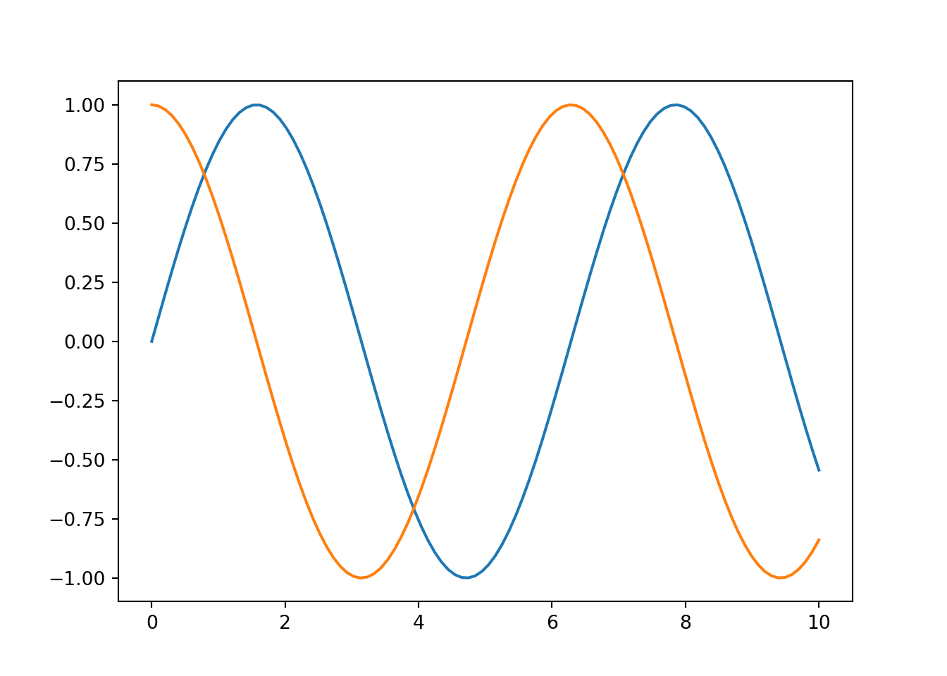
A few plots!

import matplotlib.pyplot as plt
import numpy as np
import matplotlib
matplotlib.use('Agg') # To plot with Markdown

x = np.linspace(0, 10, 100)
plt.figure();
plt.plot(x, np.sin(x))
plt.plot(x, np.cos(x))
plt.show()

plt.close()

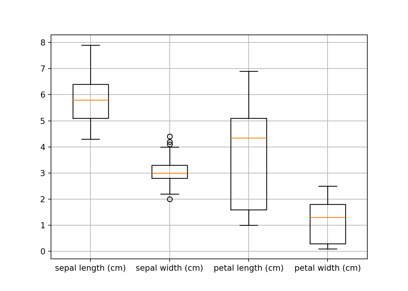
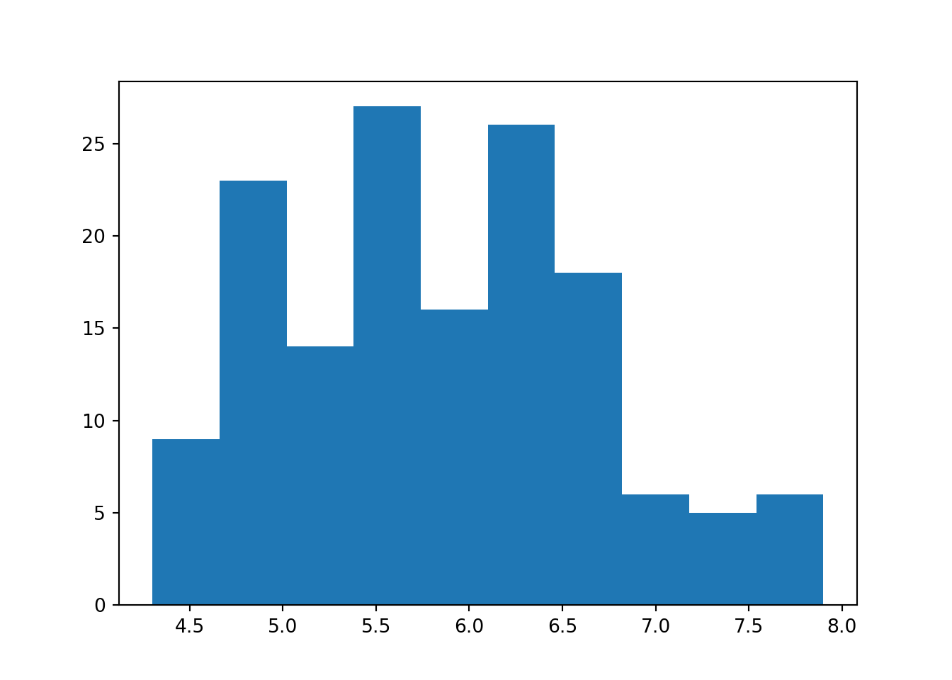
Read data from sklearn and vizualize

import matplotlib.pyplot as plt
import pandas as pd
from sklearn.datasets import load_iris 
import matplotlib
matplotlib.use('Agg') # To plot with Markdown

iris = load_iris()
df_iris = pd.DataFrame(iris.data)
df_iris.columns = iris.feature_names

# Boxplot
plt.figure();
plt.boxplot(df_iris)
{'whiskers': [<matplotlib.lines.Line2D object at 0x123089cd0>, <matplotlib.lines.Line2D object at 0x123089f70>, <matplotlib.lines.Line2D object at 0x12309afa0>, <matplotlib.lines.Line2D object at 0x1230ab280>, <matplotlib.lines.Line2D object at 0x1230b7280>, <matplotlib.lines.Line2D object at 0x1230b7520>, <matplotlib.lines.Line2D object at 0x1230c4520>, <matplotlib.lines.Line2D object at 0x1230c47c0>], 'caps': [<matplotlib.lines.Line2D object at 0x12309a250>, <matplotlib.lines.Line2D object at 0x12309a4f0>, <matplotlib.lines.Line2D object at 0x1230ab520>, <matplotlib.lines.Line2D object at 0x1230ab7c0>, <matplotlib.lines.Line2D object at 0x1230b77c0>, <matplotlib.lines.Line2D object at 0x1230b7a60>, <matplotlib.lines.Line2D object at 0x1230c4a60>, <matplotlib.lines.Line2D object at 0x1230c4d00>], 'boxes': [<matplotlib.lines.Line2D object at 0x123089a30>, <matplotlib.lines.Line2D object at 0x12309ad00>, <matplotlib.lines.Line2D object at 0x1230abfa0>, <matplotlib.lines.Line2D object at 0x1230c4280>], 'medians': [<matplotlib.lines.Line2D object at 0x12309a790>, <matplotlib.lines.Line2D object at 0x1230aba60>, <matplotlib.lines.Line2D object at 0x1230b7d00>, <matplotlib.lines.Line2D object at 0x1230c4fa0>], 'fliers': [<matplotlib.lines.Line2D object at 0x12309aa30>, <matplotlib.lines.Line2D object at 0x1230abd00>, <matplotlib.lines.Line2D object at 0x1230b7fa0>, <matplotlib.lines.Line2D object at 0x1230d2280>], 'means': []}
plt.xticks([1, 2, 3, 4], iris.feature_names)
([<matplotlib.axis.XTick object at 0x12304d430>, <matplotlib.axis.XTick object at 0x12304dc10>, <matplotlib.axis.XTick object at 0x123089700>, <matplotlib.axis.XTick object at 0x1230da070>], [Text(1, 0, 'sepal length (cm)'), Text(2, 0, 'sepal width (cm)'), Text(3, 0, 'petal length (cm)'), Text(4, 0, 'petal width (cm)')])
plt.grid()
plt.show()

plt.close()

#  histogram
plt.figure();
plt.hist(df_iris.iloc[:,0])
plt.show()

plt.close()

πŸ›Ž πŸŽ™οΈ Recordings on Canvas will cover more details and examples! Have fun learning and coding πŸ˜ƒ! Let me know how I can help!

πŸ“š πŸ‘ˆ Assignment - Python Stat/ML/Viz

Instructions are posted on Canvas.